1. Introduction to the Limits of Functions

The theory of limits is central to calculus, and so we must discuss limits of functions before we delve into differential and integral calculus. In order to discuss limits of functions we must define what a function is;

Definition 1.1: Function

Suppose we have two sets D and C. A rule that assigns to each element of D a unique element in C is called a function from D to C. The set D is called the Domain and C is called the Codomain. If $x\in D$ and $y\in C$ are related by the function $f$ we write $y=f(x)$ .

We say that x is the Independent variable and y is the dependent variable because y depends on the value of x. If $R= f(D)$ we say that R is the Range or Image of $f$ .

Limits of functions are used to describe how the function behaves when the independent variable gets close to a particular value. So taking the limit of a function say $f(x)$ as $x$ tends to some value $a$ , is essentially making a prediction for what $f(a)$ will be based on how the function behaves near $a$ . Sometimes the limits of functions do not exist for certain values and we will see why in future posts. Let’s informally look at a couple of examples to help us understand what a limit is;

Note: The value of a function $f(x)$ need not be defined at a point $a$ for $f(x)$ to have a limit there! Sometimes the limit of a function at a point is not equal to the function evaluated at that point, i.e $\lim_{x\to a} f(x)$ is not always equal to $f(a)$ .

Example 1: Consider the function $f: \mathbb{R} \to \mathbb{R}$ defined by $f(x)=x^{2}+1$ , Find $\lim_{x\to 2} f(x)$ .

By compiling a table of values for $x$ and $f(x)$ we can see how $f(x)$ behaves when $x$ is near 2.

As you can see from the table as x approaches 2 (from either side), f(x) approaches 5, and so we have $\lim_{x\to 2} f(x)$ . This is an example of when the limit at the point is equal to the value of the function at that point.

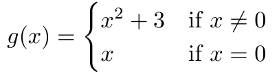
Example 2: Consider the function $g: \mathbb{R} \to \mathbb{R}$ defined by

Let’s find $\lim_{x\to 0} g(x)$ . We can do the same thing as in the last example but let’s establish the limit of this function graphically.

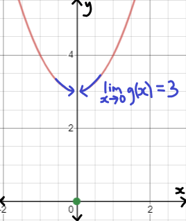
As you can see from the graph of $y=g(x)$ above, as indicated by the blue arrows, $g(x)$ approaches 3 as x approaches zero (from either side). Clearly $lim_{x\to 0} g(x)=3$ , this however, is NOT equal to the value of the function at x=0 which is $g(0)=0$ (indicated by the green dot on the graph).

The following definition is incredibly important.

Definition 1.2: Limit

Suppose that $f(x)$ is a real function (a function whose values are real numbers). If for any $\varepsilon >0$ there exists a $\delta >0$ such that for any $x$ with $|x-a|<\delta$ we have $|f(x)-L|<\varepsilon$ then $L$ is the limit of $f(x)$ as $x$ tends towards $a$ , denoted $\lim_{x\to a} f(x)=L$ .

This definition is essentially saying if $\lim_{x\to a} f(x)=L$ , then as x gets arbitrarily close to a, f(x) is also getting close to L. Our $\delta$ and $\epsilon$ is basically our mathematical way of saying how close x is to a and how close f(x) is to L respectively.

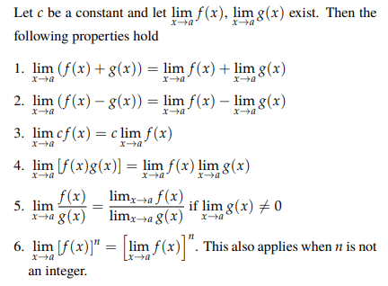
The following theorem is very important to computing the limits of functions, i will prove the first property and will leave the rest as an exercise to the reader. Feel free to send me your proofs via the contact page if you would like me to check them.

Theorem 1.1: Laws of Limits

Proof of 1.:

$lim_{x\to a} f(x)$ and $lim_{x\to a} g(x)$ both exist and so we let $lim_{x\to a} f(x)=L_{1}$ and $lim_{x\to a} g(x)=L_{2}$ . By definition 1.2 we have that for any $\varepsilon >0$ there exists a $\delta_{1} >0$ such that for any $x$ with $|x-a|<\delta_{1}$ we have $|f(x)-L_{1}|<\frac{\varepsilon}{2}$ and there exists a $\delta_{2} >0$ such that for any $x$ with $|x-a|<\delta_{2}$ we have $|g(x)-L_{2}|<\frac{\varepsilon}{2}$ .

We let $\delta = min\{\delta_{1},\delta_{2}\}$ and so $\delta$ is sufficiently small so that they both satisfy the conditions set by the limits of f(x) and g(x). Therefore

$|f(x)-L_{1}|+|g(x)-L_{2}|\geq |(f(x)-L_{1})+(g(x)-L_{2}|=|f(x)+g(x) - (L_{1}+L_{2})|$ by the triangle inequality. Now we have $|f(x)-L_{1}|+|g(x)-L_{2}|< \frac{\varepsilon}{2} + \frac{\varepsilon}{2} = \varepsilon$

and so we have $|f(x)+g(x) - (L_{1}+L_{2})|< \varepsilon$ which is precisely by definition 1.2 $lim_{x\to a} (f(x)+g(x))=lim_{x\to a} f(x)+lim_{x\to a} g(x)$ .

QED

To rigourosly show that the limit of a function is a certain value we must use definition 1.2 and establish a relationship between $\delta$ and $\varepsilon$ .

$x$	1.85	1.9	1.99	1.999	1.9999	2	2.0001	2.001	2.01	2.1	2.15
$f(x)$	4.4225	4.6	4.9601	4.9960	4.9996	5	5.0004	5.0040	5.0401	5.41	5.6225

1. Introduction to the Limits of Functions

Published by Mathsnotes

Leave a comment Cancel reply

Share this:

Related

Published by Mathsnotes

Leave a comment Cancel reply