We have seen what it means for an integer to divide another. In this post we will explore division further and delve into the idea of the greatest common divisor, seeing how this gives us information on the solubility of linear equations in the integers. I will begin by formally defining some terms formally.
Definition 2.1: Sets, Elements and the Empty Set
A Set is a collection of objects. The objects that make up a set are called the Elements of the set. The Empty Set denoted  is the unique set with no elements.
Example 2.1:
 is the set of integers,
  means that 1729 is an element of the set of integers.
 is the set of natural numbers
  .
.
Definition 2.2: Subset
Let A and B be sets. A is a Subset of B if every element of A is an element of B. This is denoted by A  B.
B.
Proposition 2.1: a|b and b|a implies |a|=|b|, i.e 
The proof of this proposition is omitted for now! This requires ring theory as we need the fact that  are the only units of the ring of integers. I will do some posts on rings in the future and will return to this proof then.
The Well-Ordering Principle is an axiom that states that every non-empty subset of  contains a least element, it is a property of the integers which is pretty intuitive.
Theorem 2.1: Given  and
and  , there exists unique integers q and r satisfying
  and
and  . q is known as the quotient and r is known as the remainder.
Proof:
We will begin by proving the existence of such a pair of integers, and then we will go on to establish their uniqueness. Let us begin by defining the set  and
and  . S is non-empty because if
  by choosing m=0 we get
  which is indeed an element of S, and if
  by choosing m=a, we get
  since
since  and
and  . We have now shown that S is a non empty set (it is easy to see that it is a non empty subset of ) which means we can now apply the well-ordering principle! So we have that S contains a least element, lets call it r. we have that
  because
  also by our construction of the set S we see that
  so
so  . All that remains for us to show (to establish existence) is that
  (we already know that
  because ). We assume for contradiction that
  and let
  , then
  and so
  ,
,  so we have
  which is a contradiction because r is the least element of S.
We now prove that the pair q,r such that a=qb+r with is unique. Assume that there is another pair of integers q’ and r’ such that a=q’b+r’ with  . Then we have a=qb+r=q’b+r’ from which we obtain (q-q’)b=(r-r’). If q=q’ then we must have r=r’ and hence we have shown uniqueness, so it suffices for us to show that q=q’. So suppose for a contradiction that
  , Then
  because
  . We have that
  but recall that and so
  which means
  which is a contradiction because |r-r’|cannot be greater than or equal to and less than b simultaneously.
QED
The theorem above is essentially saying that every integer, a, can be expressed in terms of a quotient and a remainder. This is the essence of division among the integers.
Theorem 2.2: Let  . Then there exists a unique
  and (non-unique)
  such that;
- d|a and d|b
- if
 , e|a and e|b then e|d.
 - d=ax+by (Bezout’s Identity)
Proof:
If a=b=0, then it is easy to check that we have d=0. So suppose that a and b are not both zero i.e requiring that  . Let
. Let  and
and  since S is a non-empty subset of . So we can now use the well ordering principle to establish a least element say, d>0.
  so we can write
  for some . Also by theorem 2.1 we can write a=qd+r for some
  with
with  . We want to show that d|a so assume for contradiction that
  , then
  therefore . But r<d contradicting the fact d is the least element of S, so we must have that r=0 and hence d|a. The same argument shows that d|b.
Suppose that , e|a and e|b. Then by the linearity of division (proposition 1.2) e divides any linear combination of a and b, recall that for some (i.e d is a linear combination of a and b) and so e|d.
It remains to show that d is unique, so suppose that there exists  that also satisfies 1. and 2.. Then f|d and d|f and so
  by proposition 2.1. But
  so we have d=0, thus d is unique.
QED
Definition 2.3: Greatest Common Divisor
Let , then the d given in theorem 2.2 is called the greatest common divisor of a and b, written as gcd(a,b). This is sometimes referred to as the highest common factor of a and b, hcf(a,b).
Bezout’s Identity is part 3 of theorem 2.2, here it is stated in terms of definition 2.3. Given there exist (non-unique) such that gcd(a,b)=ax+by.
Definition 2.4: Coprime
Let , we say that a and b are coprime or relatively prime if gcd(a,b)=1.
Theorem 2.3: (Euclid’s Lemma) Let  . If a|bc and gcd(a,b)=1 then a|c.
Proof:
Suppose that a|bc and gcd(a,b)=1. By Bezout’s Identity there exist such that 1=ax+by. Hence c=acx+bcy. But a|acx and a|bcy, so by the linearity of divisibility (proposition 1.2) a|(acx+bcy) which implies a|c(ax+by) i.e a|c because ax+by=1.
QED
The following theorem will show under what conditions some linear equations in the integers are soluble (i.e have a solution).
Theorem 2.4: Let . The equation  is soluble with if and only if gcd(a,b)|c.
Proof:
Let d=gcd(a,b). Then by the definition of the greatest common divisor d|a and d|b so if there exists  such that c=ax+by (i.e there exists a solution to the equation) then d|c by the linearity of divisibility (porposition 1.2). So suppose that the equation is soluble i.e that d|c. Then c=qd for some
  . By Bezouts Identity there exists
  such that d=ax’+by’. Therefore we can write c=qd=aqx’+bqy’ and so x=qx’ and y=qy’ gives a suitable solution.
QED


 means “for all elements”,
  means “there exists an element”,
  means “in the set” and
  is a set and 1, 2, 3, 4 and 5 are its elements.
 is a subset of
  assigning to each
  and
and  an element
  such that
  . We say that the set is closed
 we have
  .
. .
. we have
  .
. , where G is a non-empty set and
  ) is associative:
  .
. such that
 such that
 .
. such that
  .
. .
. , is unique.
 .
. .
. and
and  .
. and
and  .
. for all integer powers of a.
 such that
  . (if
. (if  this means
  ).
). where
where  from which we obtain b=ak. we have that b|c and so we can write this as ak|c. using the definition again we can say that
  which implies that
  and we get a|c as required. This is known as the Transitivity property of divisibility.
 such that b=an and c=am. For any
  so we have found an integer
  such that
  . Thus
  as required. This is known as the linearity property of divisibility.
 with
with  is prime if and only if its only divisors are 1 and p.
 with
with  is composite if and only if it is not prime. (i.e n=ab for some
  with
with  )
) ) and consists of 2 steps; The base case and the inductive step. The base case is the step in which we prove the statement is true for a value of n (usually n=1) . The inductive step is the step in which we link this base case to the rest of the natural numbers, we prove that if n=k is true then n=k+1, this forms a “ladder” constantly building and climbing infinitely up the natural numbers, proving the statement for all natural numbers.
  and use this to prove that it is true for n=k+1.
 with
with  , m has a prime factor (this statement is known as the inductive hypothesis) then n has a prime factor. The base case is satisfied by showing it was true for the primes i.e we have for n=4, and 1<m<4 that m is prime and the statement holds, this forms the beginning of our ladder to extend to the rest of the natural numbers. If n is composite then n=ab where
  with
with  and by the inductive hypothesis we have that a has a prime factor i.e there exists a prime p with p|a. So we have that p|a and a|n which by the transitivity property of divison implies that p|n and we have shown that n has a prime divisor.
 is a complete list of primes. Consider
  clearly by construction we have that N>1. By proposition 2, N has a prime factor p, p|N. However, every prime is supposedly one of
  , so
, so  for some
  . Therefore
  , so p|(N-1). Since we have that p|N and p|(N-1) by the linearity of divisibility (proposition 2) we have p|1 since 1=N-(N-1) which is a contradiction.
 means x does not divide y.
 where a and b are constants. (for our purposes a and b will always be integers).
 and
and  . Let
. Let  and apply Theorem 2.1 repeatedly to obtain a sequence of remainders
  defined as follows:
  where
where 
 where
where 
 where
where 
 where
where 

 we have gcd(x,y)=gcd(x+zy,y). So in terms of our remainders this is
  . Applying this over and over yields;
  where the last equality is because
  .
. (i.e. we can express the gcd of a and b as a linear combination of a and b) by ‘working backwards’. We can do this because each remainder can be expressed as a linear combination of the two previous remainders, so can the remainders before those and eventually it can be expressed in terms of a and b as we will see in the following example;


 ). Now lets work backwards to express 9 as a linear combination of 720 and 333.
 and so
 .
. , and remainders,
  , defined in the Euclidean Algorithm, we now define the sequence of integers
  , such that
  . Remember that we define
  to be the last non zero remainder and that
  . Therefore we have
  and so we set
  . Let us now explicitly define
  and
and  . So from Theorem 3.1
  and
and  and so clearly
  and
and  and so we set
  and
and  . Now for
  we recursively define by


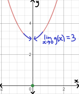
 where
where  is the axis of symmetry as shown in the following diagram;
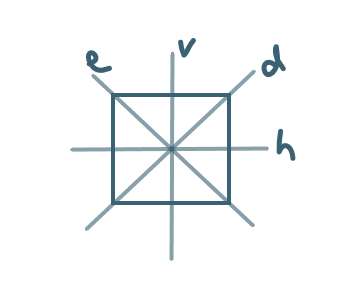
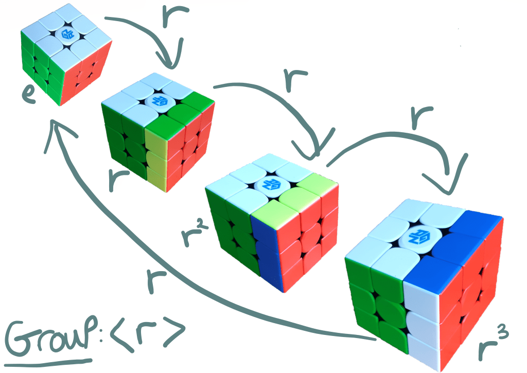
 denotes 2 of these rotations (i.e a 180 degree rotation) and
  denotes a 270 degree clockwise rotation (or equivalently a 90 degree anticlockwise rotation). Putting all of these elements together with the identity element (the action of nothing on the square) with the commutative binary operation of composition (applying the first one and then the second) forms the dihedral group denoted by
  , in the following diagram we allocate each corner a colour so that we can see how it moves with each of the elements. The dihedral groups are denoted by
  where n is the number of sides of the polygon the group is related to the symmetries of.
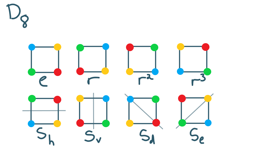

 . Take a second to convince yourself that it is closed under the composition law (composing two elements gives another element of the group), especially with respect to the reflections in the axes of symmetry.
 , the order of a is
  if there exists
  with
with  . Otherwise
  .
.


 .
. .
. where
where  . We say that “a generates G” or that a is “a generator of G”.
 is finite then
  , in otherwords the order of a cyclic group is the order of the element that generates it.
 is a cyclic subgroup of